Converting OpenCV cameras to OpenGL cameras.
28 Jun 2019This post will cover the following scenario: you have the internal and external camera calibration parameters of a hypothetical or actual camera defined in the OpenCV framework (or similar to OpenCV), and want to model this camera in OpenGL, possibly with respect to an object model.
Preliminaries and overview
The material is presented assuming that you are familiar the concepts of a pinhole camera, which is the model used for camera calibration of typical cameras in the OpenCV library. For more details about camera models and projective geometry, the best explanation is from Richard Hartley and Andrew Zisserman’s book Multiple View Geometry in Computer Vision, especially chapter 6, `Camera Models’ (this is my extremely biased view). I abbreviate that book as the “H-Z book” for the remainder of this tutorial.
This tutorial is meant to be generally self-contained, so that people can print off pages to read and make notes offline. Of course, not all sections are critical depending on your background, so skip around as needed for your own understanding.
It is possible to set many of the camera parameters using OpenGL function calls, such as glFrustrum() and glOrtho(). However, in this tutorial, I set the matrices directly, and these matrices are then sent to a shader. These details, if they are new to you, will be more clear in the code examples which are now other pages of the tutorial, starting here. Because of the direct use of matrices, this tutorial may offer some clues to derive the OpenGL projection matrices for similar camera models to the pinhole model.
Resources
These are the two resources I used for figuring out this problem. Both are great resources. If you’re here, it is likely that you see that these two resources do not spell out how to convert OpenCV calibration matrices to OpenGL matrices, which is the goal of this tutorial.
If you aren’t familiar with modern OpenGL, the below set of tutorials is a good place to start:
Roadmap
Roadmap:
- Image coordinate system differences.
- Projection in the OpenCV/H-Z framework.
- Projection in the OpenGL framework.
- Page 2: code examples
- Page 3: Rotating models with OpenGL.
Image coordinate systems in OpenCV and OpenGL
Let’s get started with some definitions!
Principal axes in OpenCV/H-Z versus OpenGL
First, we’ll discuss all the ins and outs of the image coordinate systems of the two standards.
The cameras in the H-Z and OpenCV coordinate systems both assume that the principal axis is aligned with the positive \(z\) axis. In other words, the positive \(z\) axis is pointing towards the field of view of the camera. On the other hand, in OpenGL, the principal axis is aligned with the negative \(z\) axis in the image coordinate system. Because of these changes, the \(x\) axis will also be rotated \(180\) degrees between the two representations.
Homogeneous coordinates, and Normalized Device Coordinates in OpenGL
Within the OpenCV/H-Z framework, there three coordinate frames: an image coordinate frame, camera coordinate frame, and a world coordinate frame.
Well, within the OpenGL frame, we have four: the image coordinate frame, camera coordinate frame, the world coordinate frame, and … normalized device coordinates, or NDC. I will illustrate how these work, along with the order of operations and some other needed preliminaries, by analogy with the OpenCV/H-Z framework.
Projection in the OpenCV/H-Z framework
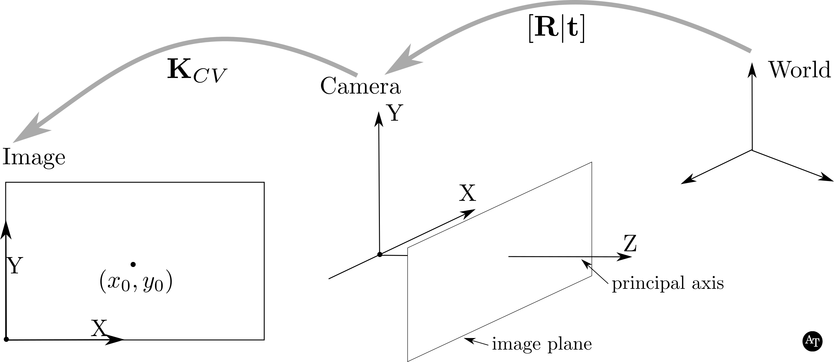
Figure 1. An illustration of the relationships between three coordinate systems: World, Camera, and Image within the OpenCV framework. Many of the ideas and basic sketch of the camera coordinate figure will be familiar for those who have well-thumbed copies of the H-Z book. The scene observed by the camera is in the direction of the positive \(Z\) axis of the camera coordinate system. In the image coordinate system, notice that the origin is in the lower left corner, and the \(Y\) axis goes up – the opposite direction of \(Y\) in the data matrix layout. More on that in Figure 3. \((x_0, y_0)\) is the principal point in the image coordinate system, and a parameter that is found during camera calibration.
Let
- \(\mathbf{K}_{CV}\): upper diagonal, \(3 \times 3\) intrinsic camera calibration matrix.
- \(\mathbf{R}\) (rotation): orthogonal \(3 \times 3\) matrix.
- \(\mathbf{t}\) (translation): column vector, size \(3\).
- \(\mathbf{X}\) (world point): column vector, size \(4\).
- \(\mathbf{x}_{CV}\) (image point): column vector, size \(3\).
Then,
\[\mathbf{x}_{CV} = \mathbf{K}_{CV}[\mathbf{R}|\mathbf{t}]\mathbf{X}\]Since we are dealing with homogeneous coordinates, we need to normalize \(\mathbf{x}_{CV}\). Assuming that the indexing for the vectors is 0-based (in other words, the first item has an index of \(0\), so the third will have an index of \(2\)):
\[\mathbf{x}_{CV} = \frac{\mathbf{x}_{CV}}{\mathbf{x}_{CV}(2)}\]Following this operation,
\[\mathbf{x}_{CV}(0) = x_{col}\] \[\mathbf{x}_{CV}(1) = x_{row}\] \[\mathbf{x}_{CV}(2) = 1\]If \(x_{col}\) or \(x_{row}\) are not within the image space, then those points are not drawn on the image. For instance, image coordinates less than zero are discarded, as are those that are larger than the image dimensions. A similar process happens in OpenGL, just add a dimension (\(z\))!
Projection in the OpenGL framework
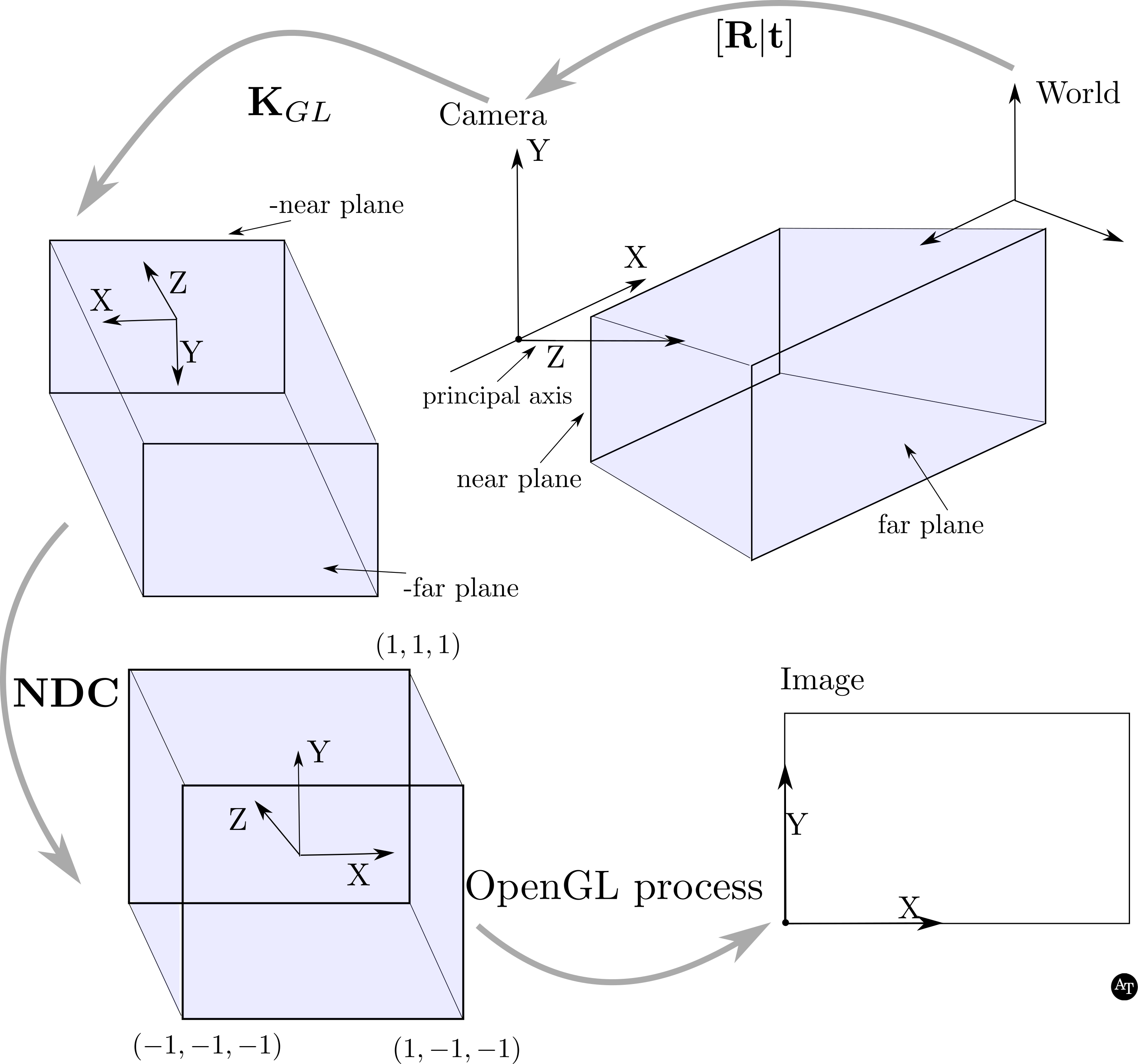
Figure 2. Importantly, note that this figure is produced for the highly specific conversion from OpenCV conventions to the OpenGL convention. Usually, the camera coordinate system has the negative \(z\) as the principal axis. If this is the case for your calibration matrices, stop, and consult other guides.
Given that we’re assuming calibration matrices where the principal axis is \(+z\) in the camera coordinate system, as in the OpenCV context the pipeline starts by transforming world points by rotation and translation \(\mathbf{R}\mid\mathbf{t}\) – exactly like in OpenCV, except with a row added to make the matrix square. Then, the camera coordinate system is slightly different; in OpenGL there is the notion of near and far planes, these are parameters that are defined by the user. The points in the camera coordinate system are transformed to the next space – I’ll call it the cuboid space – by \(\mathbf{K}_{GL}\), which is not a proper rotation and translation, but instead a reflection to a left-handed coordinate system. Then, the \(\mathbf{NDC}\) transformation transforms the cuboid space into a cube with corners that are \(\pm1\) – normalized device coordinates. This concludes all of the transformations the user has to specify – once the coordinates are in the left-handed normalized device coordinates, then OpenGL will transform those coordinates into image coordinates. To troubleshoot and transform them yourself, the equations are in Conversion Corner 1.
Let
- \(\mathbf{NDC}\) (normalized device coordinates): \(4 \times 4\) intrinsic camera calibration matrix.
- \(\mathbf{K}_{GL}\): \(4 \times 4\) intrinsic camera calibration matrix.
- \(\mathbf{R}\) (rotation): orthogonal \(3 \times 3\) matrix.
- \(\mathbf{t}\) (translation): column vector, size \(3\).
- \(\mathbf{X}\) (world point): column vector, size \(4\).
- \(\mathbf{x}_{GL}\) (image point): column vector, size \(4\).
Then,
\[\mathbf{x}_{GL} = \mathbf{NDC} \quad \mathbf{K}_{GL} \begin{bmatrix} \begin{matrix} \mathbf{R} \\ \begin{matrix} 0 & 0 & 0\end{matrix} \end{matrix} & \begin{matrix} \mathbf{t} \\ 1 \end{matrix} \end{bmatrix} \mathbf{X}\]For now, I am not going to specify the \(\mathbf{NDC}\) matrix, but instead specify how all the coordinate systems work in OpenGL. But don’t worry, we’ll get to specifying all of these items.
First, in OpenGL there is the notion of clipping points/objects that are in between the \(near\) and \(far\) planes. While in the OpenCV framework, we consider any points in between the principal plane and +infinity viewable points, this is not the case in OpenGL. To account for these planes, whereas the clipping in image space (in the previous section) is quite intuitive in OpenCV – if the point is not in the image (defined as \(\in[0, cols)\times[0, rows)\)), don’t draw it – OpenGL uses 4-element homogeneous vectors to accomplish similar aims.
I’ll denote the OpenGL NDC coordinate as \(\mathbf{x}_{GL}\); it is a column vector with \(4\) elements. It is also a homogeneous vector, and its last element is frequently given the letter \(w\). Like in the OpenCV representation, we normalize the image point \(\mathbf{x}_{GL}\) by dividing by the 4th entry (again assuming 0-based indexing); I will say that a 4-element vector is normalized when the last element is equal to 1:
\[\mathbf{x}_{GL} = \frac{\mathbf{x}_{GL}}{\mathbf{x}_{GL}(3)}\]And like before, we have a similar result:
\[\mathbf{x}_{GL}(0) = x_{NDC}\] \[\mathbf{x}_{GL}(1) = y_{NDC}\] \[\mathbf{x}_{GL}(2) = z_{NDC}\] \[\mathbf{x}_{GL}(3) = 1\]These coordinates are not necessarily image coordinates. The \(z\) values are needed so that OpenGL can compute the drawing order for objects. The NDC space is a cube of length \(2\) on each side, with dimensions \([-1, 1]\times[-1, 1]\times[-1, 1]\). Song Ho’s site has some good illustrations of the NDC space.
If any coordinate \(a\in\mathbf{x}_{GL}\) has \(\mid a\mid > 1\), then \(\mathbf{x}_{GL}\) is not drawn (or, the edge with the coordinate on the end is clipped). In other words, if any coordinate is less that -1, or greater than 1, it is outside of the NDC space.
You may have noticed that the output of the OpenGL operation is not truly an image coordinate in the sense we’re used to working with in OpenCV – in other words, a coordinate in a data matrix – and you’re right. OpenGL takes care of the conversions to image space, but it is useful to know how those work. So for troubleshooting purposes, see the box below for conversion formulae.
Conversion Corner 1
To convert from the OpenGL NDC coordinates to OpenGL image coordinates, where \(\mathbf{x}_{image, GL}\) is a 3-element vector, and \(\mathbf{x}_{GL}\) has been normalized :
\[\mathbf{x}_{image, GL} = \begin{bmatrix} cols/2 & 0 & 0 & cols/2 \\ 0 & rows/2 & 0 & rows/2 \\ 0 & 0 & 0 & 1 \end{bmatrix} \mathbf{x}_{GL}\]Note that since the image coordinate system in OpenGL is defined differently than it is in OpenCV (see Figure 3), a further conversion is needed to convert these coordinates to the OpenCV coordinates:
\[\mathbf{x}_{CV} = \begin{bmatrix} 1 & 0 & 0 \\ 0 & -1 & rows \\ 0 & 0 & 1 \end{bmatrix} \mathbf{x}_{image, GL}\]Matrices for OpenGL projection
First, use the \([\mathbf{R}\mid\mathbf{t}]\) from the OpenCV matrices, but add a row to make it square. Such as:
\[[\mathbf{R}\mid\mathbf{t}]_{GL} =\begin{bmatrix} \begin{matrix} \mathbf{R} \\ \begin{matrix} 0 & 0 & 0\end{matrix} \end{matrix} & \begin{matrix} \mathbf{t} \\ 1 \end{matrix} \end{bmatrix}\]And assuming that you have an intrinsic camera calibration matrix from the OpenCV context, \(\mathbf{K}_{CV}\), in the following form:
\[\mathbf{K}_{CV} = \begin{bmatrix} \alpha & 0 & x_0 \\ 0 & \beta & y_0 \\ 0 & 0 & 1 \\ \end{bmatrix}\]Then, we’ll use this modify the OpenCV matrix \(\mathbf{K}_{CV}\) to create the corresponding OpenGL matrix \(\mathbf{K}_{GL}\) perspective projection matrix. Note: it is highly likely that the skew parameter in the first row, second column of the OpenCV intrinsic camera calibration matrix could also be modeled in OpenGL, by negating this parameter in the \(\mathbf{K}_{GL}\) form, similarly as described in Kyle Simek’s guide. However, I have not tested this and tend to set the skew parameter to zero for my calibrations, so leave to you to test!
Given those preliminaries, and with \(rows\) and \(cols\) as the dimensions of the image, we define two new variables and the new intrinsic camera calibration matrix in the OpenGL context.
\[A = -(near + far)\] \[B = near*far\] \[\mathbf{K}_{GL} = \begin{bmatrix} -\alpha & 0 & -(cols-x_0) & 0 \\ 0 & -\beta & -(rows - y_0) & 0 \\ 0 & 0 & A & B \\ 0 & 0 & 1 & 0 \end{bmatrix}\] \[\mathbf{NDC}= \begin{bmatrix} -\frac{2}{cols} & 0 & 0 & 1 \\ 0 & \frac{2}{rows} & 0 & -1 \\ 0 & 0 & \frac{-2}{far-near} & \frac{-(far+near)}{(far-near)}\\ 0 & 0 & 0 & 1 \end{bmatrix}\] \[\quad\]Now, taking a closer look at Figure 2 and these matrices, you might be thinking, “holy smokes, why the heck would one switch back and forth, positive to negative, right-handed coordinate system to left-handed, etc., etc. Isn’t this a drag?” To which I answer: “yes.” But a couple of caveats: I am presenting the OpenGL pipeline from the perspective of someone in computer vision who loves the H-Z book and OpenCV, with a fair bit of hand-waving. In reality, and to add to the confusion, OpenGL’s camera coordinate system has as its principal axis the negative \(z\) axis. I’ll say it again in case you’ve gotten this far without seeing it – if you have matrices where the calibration assumes a negative \(z\) axis as the principal axis, check out other resources. I have done a lot of testing confirm that this works.
How can you test your camera models before getting in too deep? This is easiest with a scripting language like Matlab or octave (free), you could also do it with C++ and Eigen, Python, or any other language with which you are comfortable.
- Grab a coordinate from the world space, this could be from the object (3D model) file. This is \(\mathbf{X}\), remember this has \(4\) elements because we are using homogeneous coordinates.
- Compute the projection to the image plane in OpenCV using the matrices you have = \(\mathbf{x}_{CV}\).
- Substitute all of the values from the OpenCV matrix to the OpenGL matrices as above. Note that Matlab and/or octave are languages that start indices at 1 instead of 0 – adjust accordingly.
- If \(\mathbf{x}_{CV}\) was on the image plane, so should \(\mathbf{x}_{GL}\). If any coordinate of \(\mathbf{x}_{GL}\) is less than -1, or greater than +1 after normalization, than it will be clipped. Troubleshoot here if there are problems!
- Check that the OpenCV coordinate is equivalent to the OpenGL coordinate using the Conversions.
The data matrix layout is not the coordinate system!
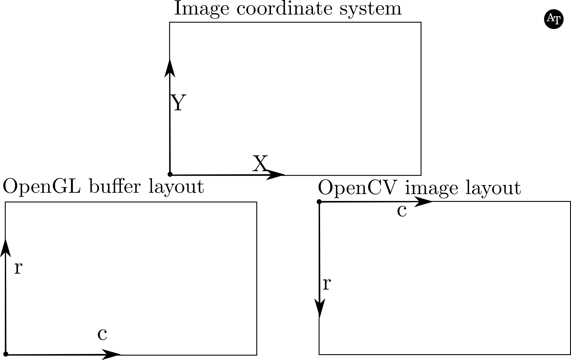
Figure 3. The top sub-figure illustrates the image coordinate system for the OpenCV and OpenGL contexts. The left lower corner shows the definition of the row (\(r\)) and column (\(c\)) indices for the OpenGL coordinate system; the OpenGL coordinate system and image coordinate system are the same (\(r=y\)). The origin for matrices in the OpenCV context is the top left corner, requiring a vertical flip of the images grabbed from OpenGL with glReadPixels( ).
Finally, I’ll end with a pedantic point concerning the layout of data matrices, in other words, the indexing of the rows and columns containing the pixels of data, and the non-relation of that layout to the image coordinate system. OpenGL has a layout different from OpenCV, which I alluded to in the Conversion Corner and the details of which are illustrated and described in the caption of Figure 3.
My code (here) currently renders the scene with OpenGL, with the correct orientation. Then, the buffer is grabbed with glReadPixels( ) and written to an OpenCV Mat image structure – upside down, so that it will turn out right-side up. The details are on Page 2.